
Fifteenth Geomechanics Lecture Geotechnical Issues in Displacement Based Earthquake Design of Highway Bridges and Walls: Part 3

Lecture Summary
There is a growing emphasis on Displacement Based Earthquake Design (DBD) analysis for buildings, retaining walls and bridge structures. DBD is specified as the preferred design method for highway structures in a draft revision of Section 5 of the Bridge Manual (NZ Transport Agency) expected to be adopted in 2016.
For bridges and major retaining wall structures, the damping and deformations within their foundations and backfilling have a major impact on their displacement response. In the past, the geotechnical input for the design of structures has focused on investigating and defining the soil strength parameters. To implement DBD methods there is now a need to investigate and assess soil stiffness as well as strength and to focus more on soil-structure interaction analysis.
The lecture highlighted the influence of soil stiffness and damping on the earthquake response of retaining walls and bridges and discussed the effects of the uncertainty in these parameters. DBD design procedures were illustrated by examples from the presenter’s research background on soil-structure interaction.
The lecture was presented in the following three parts:
- Rigid and flexible including outward sliding retaining walls
- Stiff retaining walls and bridge abutments
- Bridge DBD and pile foundations
This paper presents material discussed in Part 3 of the lecture. Material presented in Parts 1 and 2 was published in the June 2015 and June 2016 issues of NZ Geomechanics News respectively.
1. The Maitai River Bridge
Pile testing work carried out during the construction of Maitai River Bridge on State Highway 6 is described in this Part 3 of the lecture material. The bridge is also used as an example to outline the principles of DBD and to demonstrate the influence of the foundations and site subsoil conditions on the displacement response of typical highway bridges.
The Maitai River Bridge was constructed in 1988 and is located at the mouth of the Maitai River, approximately 0.6 km north of the central business area of Nelson City. The bridge has five precast prestressed concrete I beam spans with a cast in-situ reinforced concrete deck. The superstructure is supported on four piers with single 1.4 m diameter reinforced concrete columns and hammerhead type column caps. Each pier has a 1.8 m diameter cylinder foundation that consists of a reinforced concrete core cast in a 12 mm thick steel liner. The cylinders were placed by excavation and top driving of the steel shell. Typical details of the structure are shown in Figures 1 to 4.
The prestressed I beams are seated on lead-rubber bearings on both the piers and abutments that provide energy dissipation and act as base isolators to limit the lateral loads on the substructure during earthquake loading.

Figure 1: Maitai River Bridge. Looking to south.
Shear keys on the hammerhead column caps are located each side of twin transverse beams formed by diaphragms at the end of the spans. For longitudinal earthquake response there is a clearance of 75 mm between the diaphragm beams and the shear keys. In the transverse direction there is also a clear gap of 75 mm between the keys and the bottom flange of the beams. There are deck joints on the centre-line of the piers and no linkage bolts between the diaphragms either side of the joints so the spans can displace independently and hammering contact between the diaphragm beams may occur during strong longitudinal response.
The 1.4 m diameter columns are reinforced with 34 D32 longitudinal bars with a specified minimum yield stress of 275 MPa. Confinement over a 1.5 m length at the base of the column is provided by D20 hoops at 125 mm spacing. All four columns have a height of 7.62 m measured from the top of the cylinders to the top of the hammer-head pier caps. Although the bridge is base isolated, the pier columns were designed to have a relatively high resistance to lateral load and details at the base of the columns provide for moderate amounts of ductility in the unlikely event of a plastic hinge developing.

Figure 2: Elevation of Maitai River Bridge.
The main longitudinal reinforcement in the 1.8 m diameter cylinder foundations consists of 36 D32 bars (275 MPa specified minimum yield).
Four investigational bore holes were drilled to provide foundation design data. The upper sections of the foundation cylinders are embedded in unweathered to moderately weathered fine gravels in a matrix of yellowish brown silty fine sand with a trace of clay. In the upper layers the soil is medium dense with the coarser gravel layers towards the bottom of the cylinders becoming dense to very dense. The investigational work showed that the foundation soil was relatively uniform over the extent of the bridge site. A summary of the Standard Penetration Test (SPT) results is shown in Figure 5.
The bridge site is within the tidal influence of Nelson Harbour and the tops of the foundation cylinders are between 3.2 to 3.7 m below mean sea level. The maximum tidal range is about 4.0 m and thus the cylinder tops are below ground water level during the complete tidal range.
Static lateral load tests were carried out during construction of the bridge to determine the stiffness of three of the completed piers and their cylinder foundations. The maximum load applied at the tops of the piers was 325 kN which is about 41% of the load estimated to develop the ultimate flexural strengths of the columns based on estimates of probable steel yield and concrete compressive strengths.
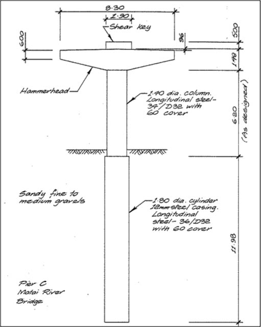
Figure 3: Typical section of the piers and foundations.
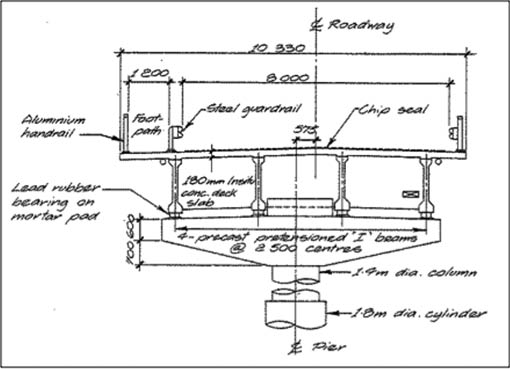
Figure 4: Typical section of the superstructure
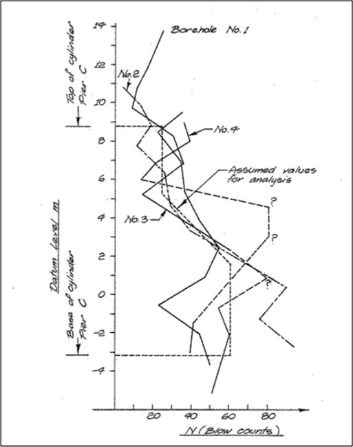
Figure 4: SPT N-values at pier pile locations
2. Maitai River Bridge Pile Testing
2.1 Loading Method
Horizontal static load testing was carried out on the piers after construction of the piers was complete and before the beams were placed on the piers. A tension loading system comprising of prestressing cables operating between the tops of adjacent piers was used. The loading system was designed to apply static horizontal loads at either the top of the pier hammerhead caps or at the base of the pier columns; however, because of the difficulties imposed by tidal waters and uneven bed levels only the pier top loading configuration was used.
Details of the pier top loading system are shown in Figures 5 and 6. The loads were applied at the top of the hammerhead of Pier C with two 25 t, 350 mm stroke jacks mounted in pairs of T shaped steel reaction frames that “hooked” on to the hammerhead and reacted against the vertical faces. Each jack and pair of reaction frames was positioned symmetrically about the column centre-line and tensioned a pair of 12.9 mm diameter Superstrand prestressing cables that had a safe load capacity of 250 kN. In order to load Pier C in a complete cycle with load reversal, cables were run to both Piers B and E and additional pairs of reaction frames were “hooked” on to both vertical faces of their hammerheads. The jacks were shifted between the two sets of loading frames each half cycle to alternately tension the cables to Piers B and E.
The cables were anchored to Piers B and E by passing them through 20 mm diameter plastic tubes cast into the hammerheads near their tops and using standard prestressing strand wedge grips.
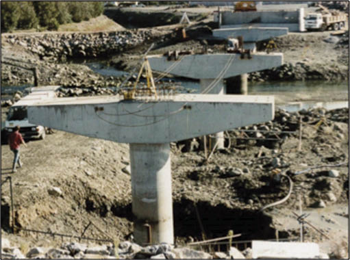
Figure 5: Cable loading system between piers.
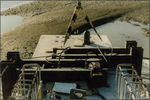
Figure 6: Loading frames on top of Pier C.
The slack in the cables was initially pulled out by hand and then by the jacks using strand wedge anchors to hold the strand temporarily against the jacking beam. The initial tension load required to remove sufficient sag in the cable spans to enable the jacks (350 mm stroke) to reach maximum load without stopping and packing was about 3.0 kN for each pair of cables.
2.2 Instrumentation
Simple instrumentation that could be installed immediately prior to the load testing was used. The loads applied by each jack were monitored by strain gauge type load cells connected to direct reading strain bridges. The accuracy of the load measuring system was of the order of 2%.
Horizontal deflections at the tops of the piers were monitored with dumpy levels positioned at distances of about 6 m from each pier and set-up to read graduated scales fastened to the hammerheads at their top surface level.
The rotation at the top of Pier C was measured with a theodolite set-up on the hammerhead to read a scale fixed to the face of Abutment A at a distance of 37.6 m from the instrument. The rotation of the top of Pier B was measured in a similar fashion using a dumpy level and a sighting distance of 19.0 m to the scale on Abutment A. The rotation and displacement scales were read to the nearest 0.5 mm.
Deflections and rotations at the tops of the piles at Piers B and C were measured using mechanical dial gauges supported from alloy reference frames held by scaffold tube posts driven into the ground on either side of the bridge centreline. The dial gauges enabled displacements of 0.01 mm to be resolved. However, because of temperature effects in the gauge support frames and creep in the loaded foundation soil it is unlikely that the displacements were recorded to better than ±0.05 mm accuracy. The accuracy of rotation measurement by the dial gauge method was of the order of ±0.07 x 10⁻³ radians.
2.3 Loading Sequence
Five complete cycles of loading were applied to Pier C by alternately tensioning the cables to Piers B and E. In the first two cycles, the loads in each direction were limited to about 60% and 90% of the maximum peak test load. The maximum peak load of 325 kN was applied in each direction of the three remaining cycles. This peak value represented approximately 75% of the theoretical load to produce first yield in the column reinforcement and was about 13% of the total dead load carried by the columns in the completed structure.
The first two of the three cycles to peak load contained six load increments and five unload increments in each of the two directions. A brief pause was made at each increment to read the instrumentation and each of these cycles took about 40 minutes to complete. The final cycle to peak load was curtailed with fewer increments because the dial gauges at the column bases had to be removed before the inflow of tidal water.
2.4 Pier Top Deflections
Deflections measured at the top of Pier C are shown in Figures 7 and 8. The plotted deflections are as recorded at the measurement point on the top surface level of the pier hammerhead.

Figure 7: Pier C top deflection. Cycles 1 to 3.
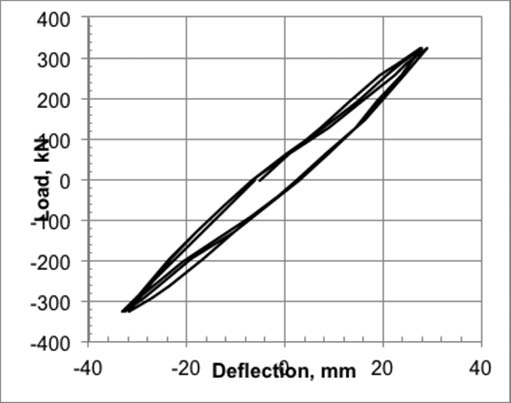
Figure 8: Pier C top deflection. Cycles 3 to 5.
A clear break in the linearity of the second loading cycle curve occurred at a load of approximately 260 kN. This change in stiffness corresponds to the load producing cracking of the concrete in the columns. On the assumption that the concrete strength in the columns at the time of testing (175 days after column pouring) was a factor of 1.5 greater than the 28 day compression test results (36 MPa), the ratio between the modulus of rupture and the compression strength at the time of test was estimated to be 0.13.
After the initial three cycles of loading, the hysteresis loops for Pier C became relatively constant in shape and the loading parts of the curves were relatively linear. A small degradation in stiffness occurred with increasing cycle number but the change is not very significant. The top deflection of Pier C in the fifth cycle, based on the average of the peak in each direction, was 31 mm. The average permanent set on release of the load in this cycle was 4 mm. The maximum top deflections of Piers B, and E in the fifth cycle were 32, and 15 mm respectively and the permanent sets in these deflections were 6, and 5 mm respectively.
2.5 Pile Top Deflections
Deflections recorded at the top of Pier C pile are shown in Figure 9. In the final three cycles of loading the Pier C pile hysteresis loops had almost constant shape with no significant degradation of stiffness. However, there was a significant permanent drift towards Pier E.
The deflection of the Pier C pile in the fifth cycle, based on the average of the peak in each direction, was 5.5 mm. The average permanent set on release of the load in this cycle was 2.2 mm.

Figure 9: Pier C pile top deflection.

Figure 10: Pier C pile top rotations.
2.6 Pile Top Rotations
Rotations recorded at the top of Pier C pile are shown in Figures 10. The rotation of the Pier C pile in the fifth cycle, based on the average of the peak in each direction, was 1 x 10⁻³ radians.
2.7 Theoretical Analyses
To provide a comparison with the test results, two analytical methods were used to compute the foundation and pier top deflections.
2.7.1 Frame Model Using Winkler Springs
In the first method a two-dimensional linear elastic frame model was used to predict the deflections of the Pier C column and pile resulting from the peak horizontal test load applied at the top of the piers. Details of the computer model are shown in Figure 11.

Figure 11: Computer model used to analyse Pier C.
The soil was modelled using Winkler springs. For the simple analysis described in the present paper linear springs were used but in other analyses described in Wood and Phillips, 1989 non-linear springs were also investigated.
Elastic moduli for concrete in the column and pile were based on measured 28 day strengths with an adjustment for the increase in strength at the time of testing at the time of testing. A cracked stiffness of the column for the column was estimated using stiffness ratios given in a chart presented in Priestley et al, 2007. The cracked stiffness is dependent on the longitudinal reinforcement and axial load ratio for the column. The pile was assumed to be uncracked and a transformed section was calculated based on the full thickness of the 12 mm thick steel shell.
SPT results obtained during the site investigation are plotted in Figure 4 together with an idealized N-value curve. This idealized curve is an approximate average of the test results and was used as the basis for determining the Winkler spring stiffness values. Firstly the N-values were increased by a factor of 1.2 to allow for the difference in driving energy between the typical New Zealand and USA penetration testing equipment. The charts of Schultze and Melzer, as published in Scott, 1981, and shown in Figure 12 were used to compute the relative density of the soil at a range of depths corresponding to the SPT N-values. The relative density was found to be approximately constant at 80% over the top 8 m of the soil profile below the top of the pile. The rate of increase of the initial tangent modulus of subgrade reaction with depth was estimated from the soil relative density using a chart from Lam and Martin, 1986 reproduced in Figure 13.
P-y curves calculated using the method described in Lam and Martin, 1986 were used to estimate the effect of non-linear behaviour and to estimate equivalent elastic springs. Curves shown in Figure 14 for the upper soil layers were calculated using a reduction factor of 1.5 on the initial tangent stiffness. This reduction factor was found to provide a good estimate of the secant stiffness in the top 2 m depth of soil.
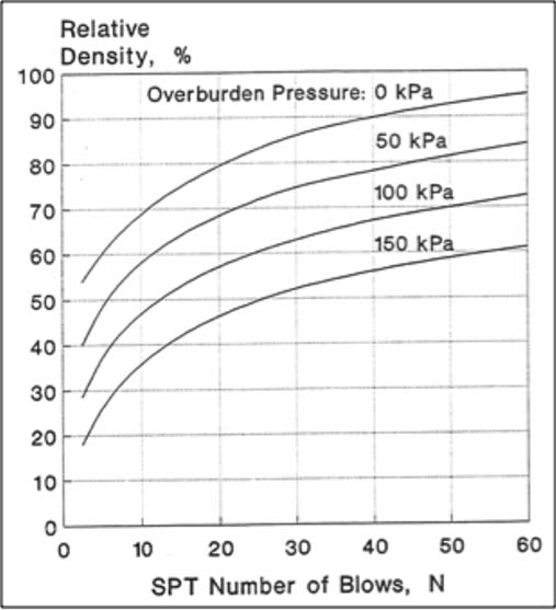
Figure 12: Schultze and Melzer curves from Scott, 1981.

Figure 13: Coefficient of subgrade reaction from Lam and Martin, 1986.
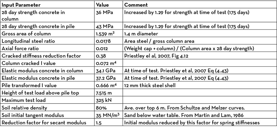
Table 1: Input Parameters for Frame Model Analysis
A summary of the main input parameters for the elastic frame model of Pier C is given in Table 1.
2.7.2 Elastic Continuum Analysis
The second analysis method was based on elastic continuum theory as presented by Pender, 1993.
For an elastic pile embedded in an elastic soil and loaded at the pile head the displacement u and the rotation q at the ground line are given by:
u = fuHH + fuMM (2.1)
q = fqHH + fqMM(2.2)
Where:
H is the applied horizontal load, M is the applied moment, and fuH, fuM, fqH, fqM are flexibility coefficients.

Figure 14: P-y curves for initial tangent modulus reduced by 1.5.
Closed form expressions are available for the flexibility coefficients in terms of Young’s modulus of the pile and soil, Poisson’s ratio of the soil and the pile diameter. For short piles, the length is also a parameter. For cohesionless soils it is often assumed that the Young’s modulus increases linearly with depth and is given by:
Es = mz (2.3)
Where:
m is the rate of increase in Young’s modulus with depth, and z is the depth below the ground line.
For a linear variation of m with depth, the flexibility coefficients are given by:
fUH = 3.2 K-333/(mD2) (2.4)
fUM = fqH = 5.0 K-0.556/(mD3) (2.5)
fqM = 13.6 K-0.778/(mD4) (2.6)
Where: K = Ep/mD
D is the pile diameter and Ep the equivalent Young’s modulus for the pile.
A value for m was estimated using the average of five equations given in Pender, 1993 for large strain Es values as a function of the SPT N-value. These equations were presented by five different research groups and are plotted in Figure 15. (Equation numbers in the legend are the number used by Pender.) The average Es at a depth of 5 m was estimated to be 48 MPa indicating an m value of approximately 10 MPa/m.
Figure 15: Plots of equations for large strain Es values. From Pender, 1993.

This value was checked using the following relationship given by Seed et al, 1985 for the small strain shear wave velocity of cohesionless soils:
vs (in m/s) = 86 Nj0.17z0.2 (2.7)
Where:
Nj is the SPT N-value as measured in Japanese practice and z is the depth below ground surface.
Because of the small power for Nj in Equation 2.7 the difference in SPT N-values from different practice can be neglected.
The small strain shear modulus Gmax is obtained from:
Gmax = r vs2 (2.8)
Where: r is the soil density.
A large strain Es value can be estimated from Gmax using:
Es = 0.4 (1+n)Gmax (2.9)
Where:
n is the Poisson’s ratio for the soil.
Equation 2.9 is based on the assumption that the large strain Es value is obtained by reducing the small strain value for the elastic constants by a factor of 0.2. This reduction factor is uncertain but is of the correct order. Equations 2.7 to 2.9 gave Es = 50 MPa at a depth of 5 m confirming that m = 10 MPa/m is of the correct order for the medium to dense sand and gravel below the water table.
2.8 Comparison of Analytical and Experimental Results
A comparison between peak measured displacements and rotations and the analytical predictions for Pier C is given in Table 2. The test displacements and rotations are given for one-half of the total peak to peak values in the fifth cycle.
Two sets of results are tabulated for each of the two analysis methods. For the frame model reducing the spring stiffness values by a factor of 2.0 was investigated. In the elastic continuum model the effect of reducing m from 10 to 9 was checked.

Table 2: Comparison of Test and Analytical Results
The frame and elastic continuum predictions based on the best estimate stiffness parameters for the soil (initial tangent modulus reduced by 1.5 for the frame model springs and m = 10 MPa/m for the elastic continuum model) are in generally good agreement with the measured results. Both analysis methods overestimated the pier top rotations by about 20%. Most of this discrepancy can be attributed to assuming a constant moment of inertia over the full height of the pier. In fact, only the lower half of the column would have been cracked and a more accurate variable stiffness model of the column would give a reduced pier top rotation.
Reducing the elastic continuum m value from 10 to 9 MPa/m gives a slightly improved prediction for the pile top displacement. Reducing the Winkler spring stiffness values by a factor of 2.0 increases the displacements at the top of the pile by approximately 60% demonstrating that although the pile steel encased section is very stiff, the pile top displacement (and rotation) are moderately sensitive to the soil stiffness assumptions
2.9 Damping
Although the test loading was applied slowly (each cycle took approximately 40 minutes to complete) it is possible to make an estimate of the hysteric damping of the pier/pile and the pile systems from the areas within the Pier C hysteresis loops which are approximately elliptical in shape (Figures 8 and 9).
The equivalent viscous damping ratio for forced harmonic vibration is given by (Priestley et al, 2007, Equation 3.10):
z = A/(2 p um Fm) (2.10)
Where:
A is the area within the force-displacement loop, um is the maximum displacement and Fm is the maximum force.
Equation 2.10 gives equivalent viscous damping for the pier/pile (pier top displacement) and the separate pile (pile top displacement) systems of 7% and 15% respectively.
Because of the influence of creep deflection in the slow static testing, the damping under dynamic loads will be less than indicated by the above estimates. However, under dynamic loads, loss of energy also occurs because of wave propagation associated with soil-structure interaction and this will tend to increase the overall damping and compensate for static creep effects.
The maximum moment applied at the base of the columns during the tests was 2,242 kN m. The flexural capacity of the column section, based on increasing the specified steel reinforcement yield stress of 275 MPa by a factor of 1.1 to give a probable yield strength of 303 MPa, was 5,990 kN m. (To calculate this value the axial load on the column was taken as the full dead load from a completed span and no strength reduction factor was applied.) The maximum test moment was therefore 41% of the flexural capacity. Greater non-linear behaviour would be expected in both the soil and column at loads corresponding to the flexural capacity of the column. This would result in higher damping than indicated by the test results.
3. Displacement Based Design of Bridges
The displacement based design procedure (DBD) has been developed-over the past 20 years (Priestley et al, 1996, and 2007) with the aim of mitigating some of deficiencies in conventional force-based design (FBD). The main difference from force-based design is that DBD characterises the structure to be designed by a single-degree-of-freedom (SDOF) representation of performance at peak displacement response, rather than by its initial elastic characteristics.
The design procedure determines the strength required at designated plastic hinge locations to achieve the design aims in terms of defined displacement objectives. It must then be combined with capacity design procedures to ensure that plastic hinges occur only where intended, and that non-ductile modes of inelastic deformation do not develop. This capacity design approach is followed in FBD but in DBD the requirements are generally less onerous than those for FBD.
3.1 Basic DBD Design Theory
The design method is illustrated with reference to Figure 16, which considers a SDOF representation of a bridge, although the basic fundamentals apply to all structural types.
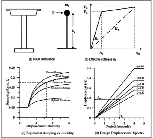
Figure 16: Main steps in DBD analysis. From Priestley, 2012.
The bi-linear envelope of the lateral force-displacement response of the SDOF representation is shown in Figure 16b. An initial elastic stiffness Ki is followed by a post yield stiffness of rKi. In contrast to FBD which characterises a structure in terms of elastic, pre-yield properties (initial stiffness Ki and elastic damping), DBD characterises the structure by secant stiffness Ke at maximum displacement Dd (Figure 16b), and a level of equivalent viscous damping representative of the combined elastic damping and the hysteretic energy absorbed during inelastic response.
In a typical DBD design procedure a trial displacement at maximum response is chosen based initially on an acceptable drift ratio or ductility level (Dd/Dy) for the structure being considered. The system damping is then determined from charts such as those shown in Figure 16c, or other published equations for structural systems or components, which give the equivalent viscous damping as a function of the ductility demand on the system or component. The effective period Te at maximum displacement response, measured at the effective height he (Figure 16a) can be read from a set of design displacement spectra for different levels of damping, as shown in Figure 16d. Design displacement spectra can be calculated from conventional acceleration response spectra (for example those given in NZS 1170.5). The effective stiffness Ke of the equivalent SDOF system at maximum displacement can be found by inverting the normal equation for the period of a SDOF oscillator to provide:
Ke = 4p2me / Te2 (3.1)
Where:
me is the effective mass of the structure participating in the fundamental mode of vibration.
From Figure 16b, the design lateral force and base shear force is:
F = Vb = Ke Dd (3.2)
A design base moment can then obtained from the lateral force F and the effective height he. The section is designed to meet his moment demand and with ductile detailing based on the assumed initial maximum plastic displacement.
The design procedure for many bridges where the mass is concentrated at the superstructure level is very straightforward with much of the effort related to determination of the substructure characteristics and determination of the design displacement. Careful consideration is however necessary in for the distribution of the design base shear force VB to the different discretized mass locations of more complex structures such as bridges with different height piers.
DBD has the merit of characterising the effects of ductility on seismic demand in a way that is independent of the system hysteretic characteristics and avoids ductility reduction factors used in FBD. The damping/ductility relationships separately generated for different hysteretic rules are available in published reports and design guidelines and there are simple rules for estimating the influence of different levels of damping on the design displacement response spectra
3.2 Design Example
A design example for the transverse response of a single bridge pier based on the dimensions and details of the Maitai River Bridge is summarised in Table 3. Because the spans are simply supported, a tributary mass approach using a single pier gives an acceptable approximation to the maximum displacement response near the centre of the bridge. To simplify the example, the displacements in the superstructure bearings at the tops of the piers have been neglected. The lead-rubber bearings used in the construction are quite flexible and provide significant damping so the calculations presented here will not closely represent the response of the as-constructed bridge. Including the bearings complicates that analysis because in this case the pier mass cannot be combined with the superstructure mass and two-mass system needs to be considered instead of the single mass used in the example.
The equation numbers listed in the comment/formula column of Table 3 refer to equations in Priestley et al 2007.
Flexibility of the foundation pile based on the test results is included in the Table 3 analysis. The sensitivity of the results to variations in these stiffness factors was investigated.
The main steps and assumption used in the example analysis are summarised below.
Structural Inputs
The structural inputs are based on the Maitai River bridge details. The span weight was taken as the weight of the superstructure plus the weight of the pier cap and one-third of the weight of the column. The effective height is the height of the centre of gravity of the total span weight with the pier cap and column weight assumed to be at the underside of the superstructure.
Foundation Stiffness Inputs
The values for pile head translation and rotation were based on the pile test results.
Earthquake Inputs
Geotechnical information for the site indicated that in terms of the NZS 1170.5 definitions the site subsoil category should be class C.
Displacement response spectra were computed from the NZS1170.5 acceleration spectra using Equation (2.2) in Priestley et al, 2007. The relationship between spectral displacement D(T) and spectral acceleration Sa(T) can be expressed as:
D(T) = T2 Sa(T)/(4 p2) (3.3)
Where:
T is the period of vibration
Displacement spectra derived from NZS1170.5 for Soil C and for 5% and 15.5% overall damping (value calculated for the example) are shown in Figure 17.
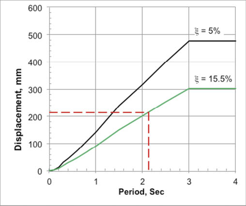
Figure 17: Displacement spectra for Soil Category C.
Yield Displacement
The yield displacement of the column was calculated from the section yield curvature which is independent of the column strength and is related to the column diameter and steel reinforcement yield strain.
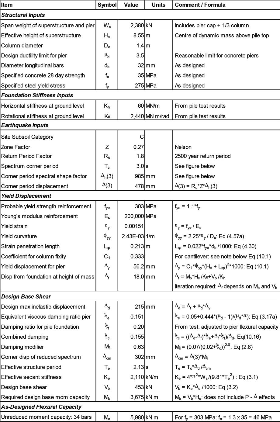
Table 3: Bridge Pier Analysis Example
The total yield displacement at the centre of mass is the sum of the column displacement and the contribution from flexibility of the foundation pile. The contribution from the pile is dependent on the column base moment and shear but at this stage of the analysis these parameters have yet to been determined. Trial and error is required to calculate the foundation displacement component. On an Excel spread sheet this can be carried out automatically using the formula iteration function.
Design Inelastic Displacement and Damping
The design level inelastic displacement was calculated from the sum of the foundation yield displacement and the total displacement in the column which is calculated from the column yield displacement and the assumed ductility capacity.
The equivalent viscous damping for the column was calculated from the assumed ductility capacity using the empirical equation given in Priestley et al, 2007. The damping in the pile/soil foundation system was increased from the value of 15% measured in the test to 20% to make allowance for the greater inelastic response expected in the soil under the applied moment and shear at the strength capacity of the column. (The moment from the test load was approximately 41% of the strength capacity of the column.)
The damping from the pier and foundation were combined using a weighted average based on displacements in the respective components. A damping modifier for the 5% damped code spectrum was calculated from the equation given in Priestley et al, 2007 (an expression first presented in Eurocode EC8, 1998).
Base Shear and Moment
The effective secant response period was calculated form the corner period of the damping reduced spectrum (15.5% damping) assuming the spectrum to ne linear over the period range from 0 to 3 seconds. This calculation is shown graphically in Figure 17.
The secant stiffness for the design level inelastic response was calculated using the SDOF expression for the relationship between period and stiffness.
The secant stiffness and the design level inelastic displacement give the required design lateral force (equal to the base shear for a SDOF structure). The required moment capacity at the base of the pier was calculated from this design lateral force and the effective height of the mass.
Column Section Details
Conventional strength or moment curvature analyses need to be carried out to determine the quantity of longitudinal reinforcement required in the column to provide the required capacity. As part of this design process the effects of P-D moments and the shear strength of the column need to be checked.
The column section in the plastic hinge region needs to be detailed with hoop confinement to provide the level of ductility assumed in the analysis. Procedures for calculating the confinement reinforcement required are given in Priestley el al, 2007. The calculations require establishing limiting strains for the steel and concrete in the plastic hinge region which are functions of the confining stress from the hoops, the volumetric ratio of the hoop steel and the strength of the confined concrete. Limit state and plastic curvatures can then be calculated from these strain limits, the section dimensions, neutral axis depth and the yield curvature (see Table 3). A plastic hinge length calculation enables the plastic displacement at the mass location to be estimated from the plastic curvature. Although the ductility calculations are straightforward, because the objective of the paper is to highlight the geotechnical aspects of DBD they are not presented here.
The ductility capacity of the pier can be calculated from the yield displacements (foundation and column) and the plastic displacement capacity of the column. The stiffness of the foundation affects the total yield displacement and since the structure ductility factor is directly related to this displacement, the foundation stiffness in turn influences the ductility capacity of the pier. Since the magnitude of the displacement spectrum is dependent on the site subsoil category the site local geology also affects the ductility capacity. Increasing the displacement demand on the pier (Soil D has a spectrum with displacements approximately 60% greater than Soil C) results in greater levels of design force and base moment and although the yield displacement in the column is unaffected by these increased demands, the yield displacement component from the foundation increases. For given set of column section properties, an increase in the yield displacement therefore reduces the pier structure ductility capacity
3.3 Parameter Study for Foundation Stiffness and Subsoil Category
The example analysis summarized in Table 3 was repeated for site subsoil Category D and for each of the two subsoil categories the required column base moment demand was computed for cases where the stiffness of the pile (lateral displacement and rotation) was increased and decreased by a factor of 2.0 (stiffness ratios of 0.5, 1.0 and 2.0). The influence of the foundation damping assumption was investigated by increasing the damping ratio (DR) from 0.2 to 0.3 for the case when the pile stiffness was assumed to be as derived from the test (stiffness ratio = 1.0).
The results of the parameter investigation are shown in Figure 18 which shows the column base moment demand for each Soil Category (C and D) and for the foundation stiffness and damping ratios investigated. The stiffness ratio shown in the figure is the ratio of the stiffness used in the analysis / the stiffness derived from the test.
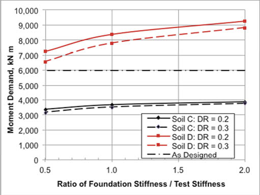
Figure 18: Moment demand related to stiffness and damping assumptions
The “as-designed” line in Figure 17 is the column base moment capacity calculated using the reinforcing in the as-constructed column and probable strengths (steel characteristic strength increased by 1.1 and concrete 28 day strength increased by 1.3).
The parameter study indicated that the base moment demand is not very sensitive to the foundation stiffness and damping ratio assumptions, particularly for the Soil C case. For the Soil D case, changing the foundation stiffness by a factor of 2.0 changes the moment demand by approximately 12%. Increasing the DR from 0.2 to 0.3 reduces the moment demand by between 5 to 10% for Soil D with the greatest decrease when the stiffness ratio is 0.5.
As expected, the subsoil category has a very large influence on the moment demand with the change from soil C to D approximately doubling the demand. It is clearly important to establish the soil category by adequate investigation and to consider interpolating between the two categories in some cases.
For this example, the as-designed columns have a moderate level of flexural reinforcement (1.8% of gross section area) and would have more than adequate moment capacity on Soil Category C but would have insufficient capacity for Soil Category D.
The total displacement and displacement components at the centre-of-mass as a function of the foundation stiffness ratio are plotted in Figure 19. The foundations contribute from 5% to 14% of the total displacement for Soil C and from 10% to 27% for Soil D. The relative magnitude of these contributions depends on the design ductility factor for the pier structure and in this case the factor of 3.5 results in quite large plastic deformations in the pier reducing the percentage contribution from the foundation. For lower structural ductility factors the foundation would have a more significant impact on the total displacements and also on the pier base moments.
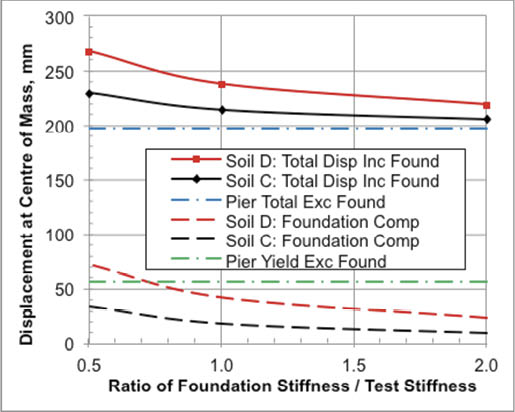
Figure 19: Total displacements and components at centre of mass
The ductility capacity of the as-designed column was checked for the range of foundation stiffness ratios investigated (0.5, 1.0 and 2.0) for each of the Soil Categories C and D. As mentioned above, the foundation stiffness and soil category influence the total yield displacement at the centre-of-mass and in this way affect the ductility capacity of the pier. Ductility capacities computed for the range of stiffness ratios investigated are shown in Figure 20. The ductility capacity is moderately sensitive to the foundation stiffness ratio and changes approximately 12% and 16% for Soil C and D respectively for a foundation stiffness ratio change of from 1.0 to 0.5 (or from 1.0 to 2.0).
The assumed ductility capacity of 3.5 in the example summarised in Table 3 would have been achieved by the as-designed section on Soil Category C. For the test pile stiffness (and less stiff foundations) more confinement reinforcing would be required than used in the design to give a ductility capacity of 3.5 for a bridge on a Soil Category D site.
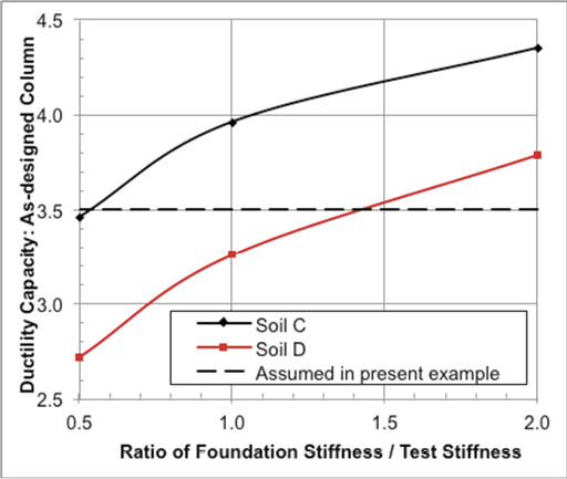
Figure 20: Ductility capacity as a function of foundation stiffness and Soil Category
In the plastic hinge zone the as-designed column had confinement reinforcing with a characteristic yield strength of 275 MPa consisting of 20 mm diameter hoops spaced at 125 mm. Reducing the hoop spacing to 100 mm would give a ductility capacity of 3.9 for a stiffness ratio of 1.0 on Soil Category D.
4 Conclusions
4.1 Pile Testing
A relatively simple static horizontal load pile test procedure followed by detailed back-analysis of the results provided valuable information on the pile foundation stiffness inputs that are important in the DBD design of highway bridges. This type of testing should be included as part of the investigation on major bridge construction projects as there is very limited published test information on the displacement performance of large diameter piles.
There was reasonably good agreement between the test and analytical predictions. However, the assumptions made regarding the soil stiffness parameters are not widely adopted in design where there may often be a tendency to underestimate the stiffness of large diameter piles in cohesionless soils. Undertaking sensitivity analyses and using several different analytical methods is an important part of any design procedure.
4.2 Displacement Based Design
Recently developed DBD procedures enable the stiffness and damping characteristics of bridge substructures to be incorporated into the design analysis is a rational and logical manner. The impact of variations in the soil foundation properties on the displacement response of a bridge can be readily established using this new approach.
A DBD example on a typical New Zealand highway bridge showed that the bridge pier flexural design was not strongly influenced by the assumptions made regarding the pile stiffness. However, the foundation stiffness will have a stronger influence on the design for low ductility factors (2.5 or less).
In the example presented the pier ductility capacity was found to be moderately sensitive to the pile stiffness assumptions.
The site Soil Category has a strong influence on the magnitude of the design displacement spectrum and in turn this has a major impact on the flexural demand and ductility detailing requirements for bridge piers. Adequate site investigation to reliably establish the local site geology is therefore important.
5. Acknowledgments
The pile testing work on the Maitai River Bridge was part of a larger project involving pile testing on four bridges. The project was financially supported by the Road Research Unit of the National Roads Board. Murray Phillips of Mills & Wood and Graeme Beattie and Bob Stevenson of the Central Laboratories of Ministry of Works and Development provided valuable assistance with the site testing work.
6 References
Bridge Manual. 2013. NZ Transport Agency. SP/M/022. 3rd Edition.
Lam I and Martin G R. 1986. Seismic Design of Highway Bridge Foundations. Vol II. Design Procedures and Guidelines. FHWA/RD-86/102. Federal Highway Administration, US Department of Transportation.
NZS 1170.5: 2004. Structural Design Actions. Part 5: Earthquake Actions – New Zealand, Standards, New Zealand.
Pender M J, 1993. Aseismic Pile Foundation Design Analysis, NZSEE, Vol 26 No 1 pp 49 – 161.
Priestley M J N. 2012. Displacement-Based Seismic Design of Bridges. Presentation at NZBridges Conference, Wellington.
Priestley M J N, Calvi G M and Kowalsky M J. 2007. Displacement-Based Seismic Design of Structures, IUSS Press.
Priestley M J N, Seible F and Calvi G M, 1996. Seismic Design and Retrofit of Bridges. John Wiley & Sons Inc.
Scott R F. 1981. Foundation Analysis. Prentice-Hall Inc, New Jersey.
Seed H B, Wong R T, Idriss I M, and Tokimatsu K. 1986. Moduli and Damping Factors for Dynamic Analysis of Cohesionless Soils. ASCE, Geotechnical Eng., Vol 112, No 11.
Wood J H, Phillips M H. 1988. Lateral Load Stiffness of Bridge Pile Foundations: Load Tests on Maitai River Bridge. Report ST88/1, Mills & Wood. Report to Road Research Unit, National Roads Board.

Save