Development of a magnetic tracking system for monitoring ground movements during geohazards: some preliminary results
Abstract
In the study of geotechnical hazards, such as soil liquefaction and landslide, the analysis of soil movements or soil particle movements is always one of the major preoccupations. An efficient soil movement sensing technique requires the tracking of different parts of a soil mass in order to develop an overall displacement field for the purpose of examining the mechanism involved and to establish a precise early warning system. A magnetic tracker system is therefore proposed with permanent magnets as trackers and magnetometers as receivers. When permanent magnets, deployed in soil to serve as excitation sources, move with a soil body during a geotechnical event, they generate static magnetic fields whose flux densities are related to the positions and orientations of the magnets. Magnetometers are used as receivers to detect the generated magnetic fields, which can be further used in calculating the magnets’ locations and orientations based on appropriate algorithms. Due to the fact that soil has magnetic permeability very similar to that of non-ferromagnetic materials, such as air and water, it cannot influence the static magnetic field generated by magnets; therefore high accuracy can be guaranteed within a limited sensing range. This paper presents some of the results of preliminary works on the use of magnetic sensing technology for ground deformation detection.
1 INTRODUCTION
Identification of possible failure mechanisms and assessment of potential damage associated with earthquake hazards are important ingredients in mitigating their impacts to the built environment (Orense 2003). Understanding “why” and “how” these hazards will occur can help engineers and public policy makers design safer structures and sites for the society. On the other hand, there is also a need to assess the temporal development of failure, i.e. to evaluate “when” ground failures will occur and their progress, so that countermeasures and necessary operations to reduce damage can be effectively implemented. One way to achieve this is through monitoring and alarm systems.
Monitoring ground deformations is a vital component of many early warning systems that have been established. Such systems require continuous recording of soil movements, so that if the monitored movement reaches a pre-set threshold, precaution of failure (such as warning or alarm) is generally issued. Moreover, accurate tracing of the exact movements of soil particles can shed further understanding of the mechanism of the seismic hazard and the consequent countermeasure techniques. For example, understanding the mechanism of subsurface ground deformations induced by soil liquefaction could provide better insight on the mechanism(s) involved in the process for better design of underground structures.
Although significant progress concerning soil liquefaction has been achieved through a large number of high quality field investigations, almost all of the findings so far relate to the displacements observed on the ground surface, i.e. the cause of and the mechanism behind seismically-induced ground surface deformation remains unknown. Delicately designed laboratory tests can simulate this very well, but because of the opaqueness of the soil grains, the exact particle movements within a soil model is difficult to quantify. For this reason, other methods of monitoring subsurface deformation that can withstand underground condition (presence of soil cover, saturated soil environment, etc.) need to be developed.
In general, movement sensing can be categorise into two groups: positioning sensing and displacement sensing (Nyce 2004). In positioning sensing, the distance between a reference point and the present location of the target is measured. For example, in landslide monitoring, an extensometer can be used to measure changes in the length of a slope; a long wire and a fixed pole is necessary to measure the distance between the pole and the target location. Although a non-contact extensometer may not need long wires to measure distance, fixed points are still indispensable. Conversely, in displacement sensing, the distance between the current location and the previously recorded location is measured. For example, an inertial navigation system (INS) is a relative measurement which does not rely on external fixed point. Akeila et al. (2007; 2010) used smart pebbles embedded with a strap-down INS system to monitor riverbed sediment transport. Although these smart pebbles can also be applied in soils to record information related to acceleration and applied forces, the most important displacement information is beyond capture. To circumvent this, the exact position of a target in three-dimensional space can be calculated mathematically by integrating the accelerations and rotations about the three axes; however, since the data are error-prone, the integration processes lead to errors that grow with time (Paik 1996). A Global Positioning System (GPS)-aided INS can be applied in the smart pebble to increase the level of accuracy and reliability as well as the information update rate. However, as the targets of interest are usually buried, which means the signals of smart pebble underground need to penetrate the depth of soil without being blocked, the strength of the signal may not be strong enough to guarantee the accuracy.
In order to overcome the shortcomings described above, a novel way of monitoring ground deformations is examined. In this paper, the technology whereby soil movement can be obtained from a magnetic sensing technique is introduced. Firstly, the algorithm developed to define the location and orientation of the magnets is discussed and its validation using a numerical model is presented. Finally, the results of simple physical model tests are presented as a way of illustrating the capability of the proposed technique.
2 MAGNETIC SENSOR SYSTEMS
2.1 Background
Magnetic sensor system is a type of position sensing technique with an obvious advantage of non-contact operation. When a permanent magnet (acting as magnetic tracer) is deployed within the subsoil, it will generate a magnetic field which can be detected by magnetometers (magnetic field sensors) above the ground. The magnetic strength and direction at a certain target point in the ground give information about the relative distance between the target point and the magnetic tracer. As soil moves during an earthquake and/or liquefaction, the magnetic tracer will move along with the soil particles (provided they have similar density). In this way, the movements of the soil particles can be traced by the movements of the magnetic tracer.
The position as well as the direction information can be derived by detecting the magnetic flux density (B with the unit of Tesla) around the magnetic dipole. Schlageter et al. (2001) developed a system capable of tracking a permanent magnet with a 2D-array of 16 cylindrical Hall sensors. Hu et al. (2006) investigated the use of magnet-based localization in wireless capsule endoscopic technique. Also, because soil has magnetic permeability very similar to that of non-ferromagnetic materials, such as air and water, it cannot influence the static magnetic field generated by magnets. Therefore, it is possible to locate a magnetic tracker buried in soil with high accuracy. When the magnetic tracker is deployed in soil, it will generate a magnetic field which can be detected by magnetometers. The magnetic flux density at a certain target point in the space gives information about the relative distance between that target point and the magnetic tracker. As soil moves due to geohazards, the magnetic tracker will move along with the soil particles. In this way, the movements of the soil particles can be illustrated by the movements of the magnetic tracker.
There are some advantages of the magnetic tracer technique compared to other existing techniques: (1) there is no way to block a magnetic field, so this tracing technique has the potential to be well-applied underground; (2) the feasibility of accurate tracing is largely dependent on the strength produced by the magnetic tracer; so if the strength of a permanent magnet mixed with soil particles can be strong enough, the size of the tracer can be as small as a normal permanent magnet due to the fact that no other circuits or devices are required (unlike the smart pebble); although in order to enhance the field strength of a tracer, an electromagnet with batteries can be installed together as a tracer.
2.2 Formulation of Algorithm
The first step in the research concerning the establishment of the magnetic sensor system is to come up with an algorithm to calculate the location information about a tracker (or multiple trackers) from data collected by magnetometers. Each set of data collected by a magnetometer at a specific point is comprised of three-axis magnetic flux densities. The proposed algorithm can calculate the coordinate point (x, y, z), using the magnetic flux densities.
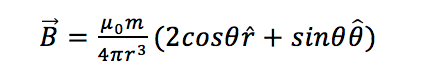
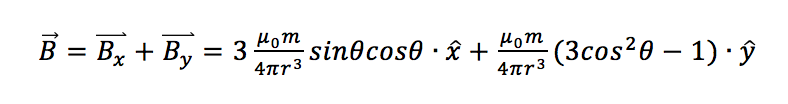
The proposed magnetic sensor system comprises permanent magnets as trackers, and magnetometers as receivers to detect the magnetic flux densities generated by the trackers. Trackers are buried in soils and magnetometers are arranged outside the soil body of interest. Collected data is sent to a computer and then analysed through proper algorithm to determine the locations of the trackers. The relationship between the magnetic flux density at a spatial point and the location of the point is illustrated by:
 (1)
(1)
 (2)
(2)
where is the magnetic moment of the dipole whose unit is; is the permeability of a vacuum (free space), and is measured in Tesla. The values of and provide the information of the location of the magnetic tracker in polar coordinates. and are unit vectors shown in Figure 1. Although the above equations are easy to understand, it is difficult to develop an effective algorithm based on the above equations because during any movement, the direction of the tracker or the direction of the magnetic moment is not constant.
Figure 1: Schematic of the magnetic flux density generated by a magnetic dipole
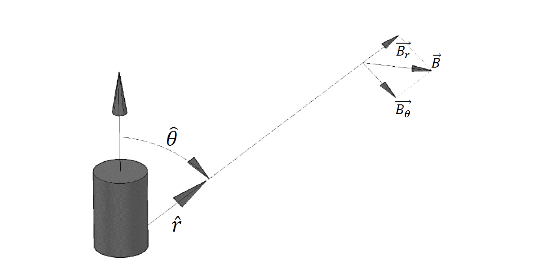
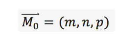
In reality, the magnetic flux density at a spatial point is not only dependent on the relative distance from the magnet, but also dependent on the orientation of the magnet (the magnetization direction). To solve the location (x, y, z) and the orientation (m, n, p) of a tracker, 6 independent equations are required. However, considering that the size of the tracker is much smaller than the distance between the tracker and the magnetometers and the tracker is either a disc magnet or an electromagnetic coil, spinning around the axis of the magnetization direction will not change the spatial distributions of the magnetic flux densities. Hence, the magnetic positioning in this case is actually a 5-D positioning because, in addition to 3 unknowns related with location, there are only 2 more unknowns required to indicate the orientation. As a result, it is more convenient to change the above equations into the following ones including a unit vector indicating the direction of the magnetic dipole:
 (3)
(3)
 (4)
(4)
 (5)
(5)
 (6)
(6)
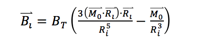
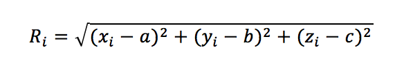
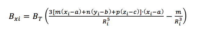
where is a constant parameter related to the magnet being used; is the magnetic flux density detected by magnetometer , where the location of the magnetometer is indicated by ; denotes the magnetization direction of the magnet with ; and is the location of interest. The schematic of the magnetic sensor system is shown in Figure 2. In order to develop the algorithm required, Equation (3) can be expanded as:
 (7)
(7)
 (8)
(8)
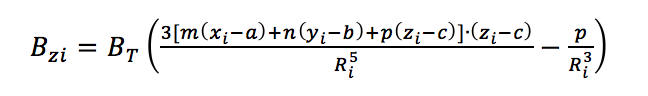 (9)
(9)
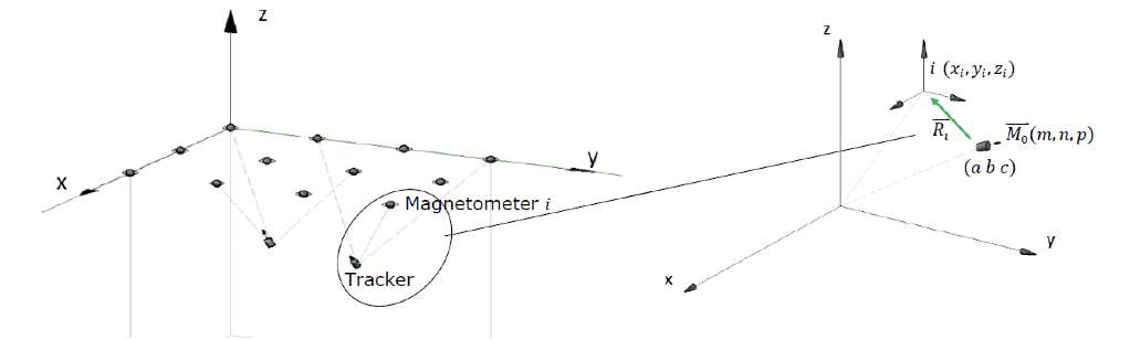
Figure 2: Schematic of the magnetic sensor system in the global coordinate frame.
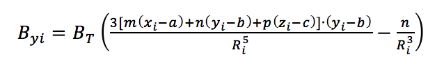
where Bxi , Byi and Bzi are the x, y and z components of respectively. An effective algorithm should be able to solve the equations for the position of the tracker and the orientation using the inputs of, and , and also with the known position of the magnetometer . In order to solve the above high-order nonlinear equations, a Levenberg-Marquardt (L-M) algorithm (Levenberg 1944; Marquardt 1963) and a linear algorithm are used (Hu et al., 2006). Due to space limitation, the appropriate equations for these algorithms are not presented here; however, both linear and L-M algorithms can be coded easily in MATLAB.
3 VALIDATION OF ALGORITHM
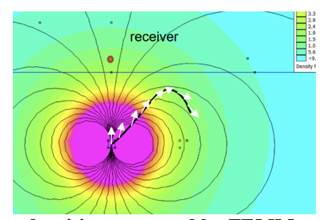
In order to test the algorithm without data derived from real physical tests, Finite Element Method Magnetics (FEMM) (Meeker, 2015) was used to generate the magnetic flux density from a permanent magnet (10 mm , 10 mm high, 52 MGOe Neodymium magnet). In FEMM, a permanent magnet is modelled as a volume of ferromagnetic material surrounded by a thin sheet of current. Assuming the locations and directions of magnetization of the permanent magnet change as shown by the white arrows in Figure 3, the two-axis magnetic flux densities are recorded at the location of the receiver each time it moves. White noise is then added to the recorded flux densities to simulate the real ones captured by a magnetometer. As shown in the figure, the movement of the tracker is assumed as
 (10)
(10)
 (11)
(11)
Figure 3: Magnetic flux densities generated by FEMM as assumed inputs
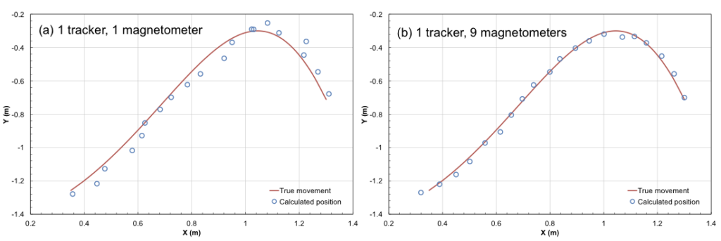
The algorithm developed is tested in the MATLAB program in a 2-D scenario, which uses magnetic flux density , and generated by FEMM with some additional white noise. As shown in Figure 4, the more magnetometers being used, the more accurate the location would be, and even with only one magnetometer, the algorithm can provide acceptable results. However, when using the L-M method to solve non-linear high order equations, a starting point or an initial guess is required to begin iteration, and if the initial guess has large error, the algorithm may fail to give correct global minimizer due to the fact that there are too many local minimizers.
Figure 4: (a) L-M method tested with 1 magnetometer and one tracker; (b) L-M method tested with 9 magnetometers and one tracker.
The linear algorithm is also tested in the MATLAB program in a 3-D scenario. For the linear method, at least 6 magnetometers are required for tracking 1 magnet in space. Compared to the L-M method, an advantage is that there is no need for an initial guess to be set. However, the number of magnetometers required increases as the number of trackers increases. Moreover, the linear algorithm cannot be used in 2-D scenario, because the coplanar assumption is automatically satisfied in 2-D. Due to space limitation, the validation for linear algorithm through FEMM is not shown here.
4 VALIDATION THROUGH PHYSICAL MODEL TESTS
Preliminary physical tests are conducted in two sequential steps. In the first step, the magne-tometers are calibrated in a real sensor array system before using to collect data. Secondly, the combination of the linear algorithm and the Levenberg-Marquardt algorithm is tested.
4.1 Calibrations of magnetometers
A magnetometer is a type of sensor that measures the strength and orientation of local magnetic flux density. Due to the fact that magnetic measurements are subjected to hard and soft iron distortions, all readings from the three axes of a magnetometer should be calibrated before use. Hard-iron distortions are produced by nearby materials, such as a permanent magnet or a piece of magnetized iron, that generate a magnetic field superimposed on the earth’s magnetic field. Therefore hard-iron distortions usually result in a permanent bias in the sensor readings. On the other hand, soft-iron distortions are created when there are ferromagnetic materials nearby, which are not necessarily the sources of magnetic fields but will influence or distort local magnetic field.
However, in magnetic localization of a magnetic tracker, it is the change of the detected magnetic field that can be used to calculate the relative locations of the tracker. Consequently, it is only necessary to find out the gains (or sensitivities) of all the three axes of each magnetometer. For example, in the x-axis readings of Magnetometer No. i, the relationship of the sampled data and the location information, as well as the orientation information, can be represented by Equation (12):
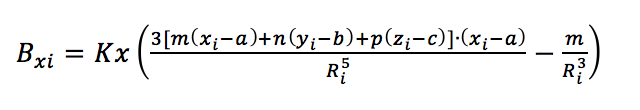 (12)
(12)
where is the sampled data by x axis from Magnetometer No. i, while is the sensitivity of that axis. Other parameters are same with those in Equations (3) to (9). In order to acquire the sensitivity of x axis of magnetometer No. i, a permanent magnet is moved along the magnetometer x axis on the line where y and z components are 0, such that and . During calibration, sampled data and displacements between magnet and magnetometer () are recorded. Therefore, sensitivity is derived as:
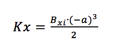 (13)
(13)
For higher accuracy, 11 samples are taken for calibration of each axis. For each magnetometer used, the sensitivities in x-, y-, and z-directions were evaluated.
4.2 Test results
After proper calibrations, 9 magnetometers were arranged in an array, as shown in Figure 5. In the first series of tests, in order to verify the feasibility and to evaluate the errors of calculation, a laser sensor is used to detect the displacement of a permanent magnet moving linearly. In the first trial, the permanent magnet was set lying down so that the orientation is parallel to the direction of movement, i.e. the orientation remains constant at around (0, -1, 0). In the second trial, the magnet was maintained upright such that its movement was perpendicular to its orientation, which is (0, 0, 1). In the second series of tests, the movement of the permanent magnet undergoing pendulum movement was investigated. In all cases, the magnetometers sampled data every 0.1 sec. Note that due to the limited effective range of the laser sensor, the total displacement of the permanent magnet (the tracker) in the first series of test was limited to 20 cm. Figure 6(a) shows the results detected from magnetometer array compared to that using laser sensor for the first trial, while the results for the second trial are shown in Figure 6(b).
Figure 5: Sensor layout in the first model test.
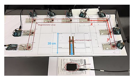
Figure 6: Comparison of movement from sensors and laser: (a) Trial 1; and (b) Trial 2
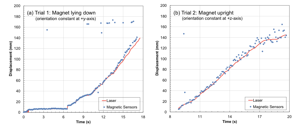
It can be seen from the results that the magnetic sensing system detected the position of the moving magnet quite accurately. The difference between the results is that when the magnet remained upright, the vertical components of magnetic flux densities at the locations of the magnetometers were dominant as compared to the horizontal components, because the magnet was moving on the same plane where those magnetometers were located. As a result, for all the 27 sets of data input (i.e. 3 for each magnetometer), only 9 (all the z-axis) of them have the great impact on the calculation.
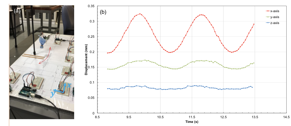
The second test was conducted with the magnet wrapped by a piece of cloth and allowed to swing, like a pendulum. The experimental set-up is shown in Figure 7(a). The high speed spinning of the magnet was prevented and it swung generally along the x axis. Figure 7(b) shows the three axis projections of its movement versus time. The results show that the algorithm developed generally tracked the sinusoidal movement of the magnet very well in the x direction. Since the movement was not really confined to along x-axis only, similar sinusoidal movement, albeit with smaller amplitude, can be observed on the y-axis. Along z-axis, movement was generally negligible.
Figure 7: Pendulum test: (a) experimental set-up; (b) results
5 CONCLUDING REMARKS
The feasibility of using a magnetometer array to locate a magnetic tracker (e.g. a permanent magnet) is proved to be possible, as illustrated by the simple physical model tests. Future improvements of the accuracy of the magnetometer array can be achieved by: 1) further calibration such as magnetometer position adjustment and magnetometer orientation adjustment; and 2) rearranging the magnetometers to reach an optimized arrangement, in which the potentials of all three axes of those magnetometers can be exploited to the hilt. Moreover, it is planned in the future to perform small-scale laboratory tests where the permanent magnet will be buried in moving ground, simulating landslides and/or lateral flow of liquefied soil.
6 ACKNOWLEDGMENT
The authors would like to acknowledge the assistance of staff of the Dept. of Electrical and Computer Engineering, University of Auckland, particularly Dr Dariusz Kacprzak for providing guidance in understanding FEMM and Rob Champion, for the assembly of the magnetometers.
REFERENCES
Akeila, E., Salcic, Z., Kularatna, N., Melville, B. and Dwivedi, A. (2007) Testing and calibration of smart pebble for river bed sediment transport monitoring. Proceedings of IEEE Sensors, Art. No. 4388624, 1201-1204.
Akeila, E., Salcic, Z. & Swain A. (2010) Smart pebble for monitoring riverbed sediment transport. Sensors Journal, IEEE, 10(11), 1705-1717.
Hu, C., Meng, MQ-H. & Mandal, M. (2006) Efficient linear algorithm for magnetic localization and orientation in capsule endoscopy. 2005 IEEE Engineering in Medicine and Biology 27th Annual Conference.
Levenberg, K. (1944) A method for the solution of certain non-linear problems in least squares. Quarterly of Applied Mathematics 2.2: 164-168.
Marquardt, D. W. (1963) An algorithm for least-squares estimation of nonlinear parameters. Journ. Society for Industrial and Applied Mathematics 11(2): 431-441.
Meeker, D. (2015) Finite Element Method Magnetic, User’s Manual Vers 4.2.
Nyce, D.S. (2004) Linear Position Sensors: Theory and Application. John Wiley & Sons.
Orense, R.P. (2003) Geotechnical Hazards: Nature, Assessment and Mitigation, University of the Philippines Press, 510pp.
Paik, H.J. (1996) Superconducting accelerometers, gravitational-wave transducers, and gravity gradiometers. SQUID Sensors: Fundamentals, Fabrication and Applications (H. Weinstock, Ed.) Kluwer, 569–598.
Schlageter, V., Besse, P.-A. , Popovic, R.S. & Kucera, P. (2001) Tracking system with five degrees of freedom using a 2D-array of Hall sensors and a permanent magnet. Sensors and Actuators A: Physical, 92(1): 37-42.