Abstract
Routine effective stress analyses for failure of geotechnical structures use a linear Mohr-Coulomb envelope and routine analyses for ground movements use linear elasticity with constant Young’s Modulus E’ or one-dimensional modulus M’. Observations of soil behaviour show that strength and stiffness are non-linear and so the conventional simplifications do not match these basic observations. Measurements from several different soils show that their strengths can be represented by a simple power law similar to the familiar Hoek-Brown model for rock strength. For soft soil, stiffness for analyses of settlements of embankments may be approximated as linear. For stiff soil which is highly non-linear, a value of E’ for analyses of settlements of foundations may be approximated to E’0/3 where E’0 is the stiffness at very small strain.
1 SOIL STRENGTH
1.1 Conventional Linear Mohr-Coulomb Soil Strength Envelope
A linear relationship between the limiting shear force and normal force is attributed to Coulomb (1773) as discussed by Heyman (1972). Following the development of analysis of stress by Mohr the original Coulomb relationship was recast in stresses and this is the familiar Mohr-Coulomb strength criterion. In the original Mohr-Coulomb strength criterion stresses were total stresses and the relationship was mostly applied to unsaturated compacted fills. Terzaghi (1936) extended the original Mohr-Coulomb criterion to effective stresses and this is now the conventional criterion for soil strength.
(a)
(b)
Figure 1: Mohr-Coulomb linear soil strength envelopes
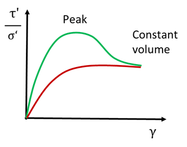
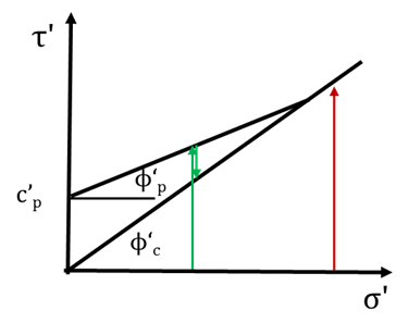
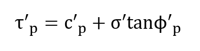
In Figure 1(a) a typical stress –strain curve for soil has a peak strength at a strain of the order of 1% and a smaller constant volume or critical state strength at a strain of the order of 10%. (Clay soils may also have a lower residual strength after very large deformations on a slip plane.) It is well established that all these strengths increase with effective normal stress and they are conventionally described by linear relationships as shown in Figure 1(b) so the peak strength is given by
Equation 1
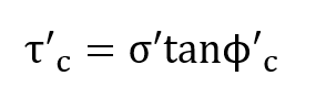
and the constant volume or critical state strength is given by
Equation 2
It is also well established that at sufficiently large normal stresses soils do not have a peak strength only a constant volume strength so the peak and constant volume failure envelopes must meet as shown in Figure 1(b). The stress paths in Figure 1(b) correspond to the stress ratio strain curves Figure 1(a).
In conventional geotechnical engineering practice the linear Mohr-Coulomb strength envelope is used for routine analyses of ultimate limit states with a factor of safety of about 1.3 and it is used for routine assessment of serviceability limit states with a load factor of about 3.
1.2 Peak strength of soil
Figure 2 shows a set of Mohr circles for the stresses at the peak state and the constant volume, critical state of samples of London Clay (Atkinson and Crabb 1997). The constant volume envelope shown by double lines is linear with parameters c’ = 0 and ϕ’c = 220. The circles for the peak states have a curved envelope which passes through or very close to the origin. It should be noted that the stresses in the samples with the lowest stresses were only a few kiloPascals requiring very careful experimental techniques.
Figure 2: Failure envelope for London clay
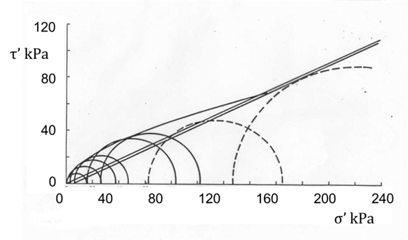
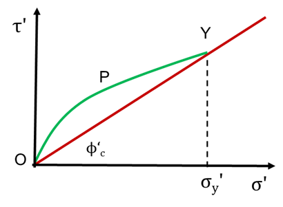
Figure 3(a) illustrates the features of the peak envelope from Figure 2. The effective stress strength is negligible when the effective normal stress is zero at the point O. It is impossible to make a stable vertical slope in dry sand. In plastic clays the strength at zero effective normal stress may not be exactly zero but careful experiments show that it is very small and only a few kiloPascals (Atkinson 2007). At relative large effective normal stresses beyond the point Y soils have no peak strength only a constant volume strength. Between O and Y there is a peak strength at P which is larger than the constant volume linear strength envelope. It is impossible for a linear peak strength envelope to join the points O – P – Y.
It is worth recalling that Coulomb developed the linear relationship for unsaturated compacted fill in military earthworks (Heyman 1972). For such soils, and in total stresses, there is a substantial strength at zero total stress. Although the relationship between strength and total normal stress may not be exactly linear the original Mohr-Coulomb total stress relationship is not obviously incorrect for unsaturated soils. It was when the original total stress linear criterion was converted to effective stress by Terzaghi (1936) that it no longer correctly represented observed behaviour of saturated soil.
1.3 Non-linear soil strength
A convenient formulation for the non-linear peak envelope in Figure 3(a) is a simple power law such as
Equation 3
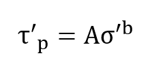
where A and b are parameters that depend on the soil grains and on the critical stress σ’y. This simple power law is similar to the basic formulation of the Hoek-Brown (1980) criterion commonly used to describe the strength of rock. A similar power law was found by Atkinson (2007) for peak strengths of several overconsolidated clays.
(a)
(b)
Figure 3: Non-linear soil strength envelopes
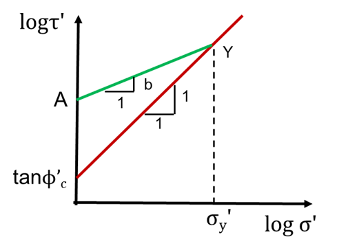
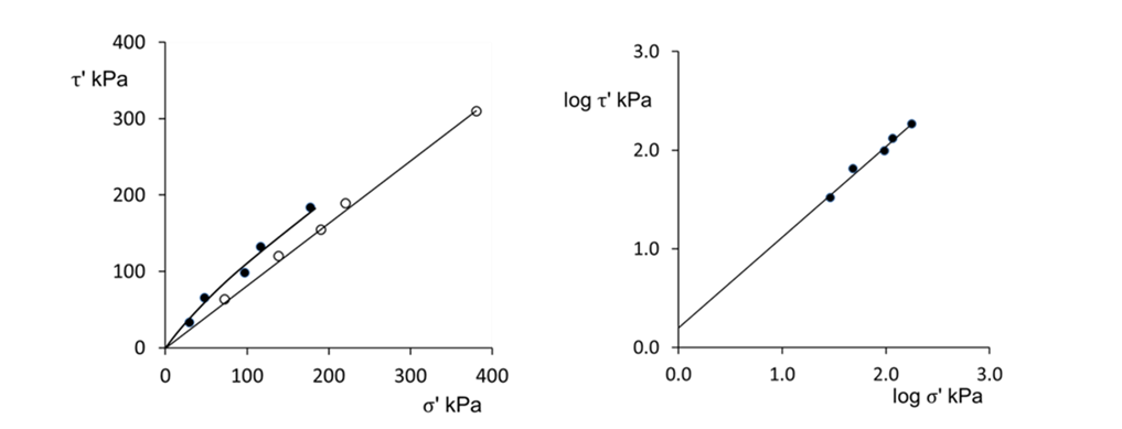
When the stresses are converted to logarithms equation 3 becomes
Equation 4
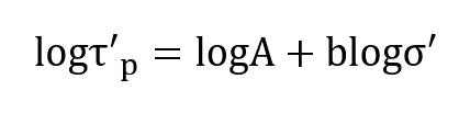
which gives a log-linear envelope as shown in Figure 3(b). Figures 4(a) to (d) show peak and constant volume strengths of some fine and coarse grained soils.
(a) Kaolin clay
(b) Glacial till
(c) Carbonate sand
(d) Quartz sand
Figure 4: Peak and constant volume strengths of soil
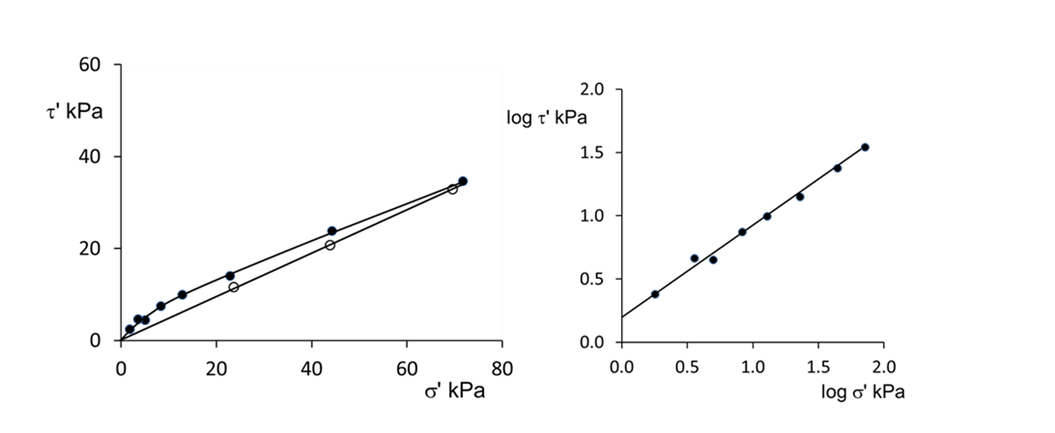
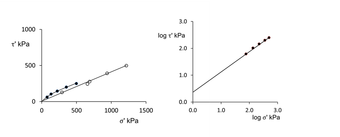
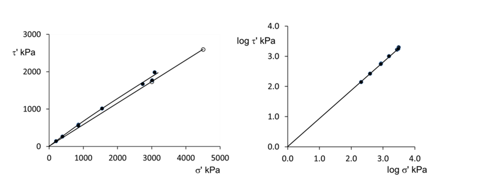
In the left hand diagrams in Figure 4 the constant volume critical state strengths are linear with arithmetic scales and conform to equation 2. In the right hand diagrams the peak state strengths are linear with logarithmic scales and conform to equation 4. Values for the parameters A and b in equation 4 and the constant volume friction angle ϕ’c in equation 2 are summarised in Table 1.
Table 1: Values for parameters in Figures 4
Soil A b ϕ‘c Kaolin clay 1.6 0.72 25 Glacial till 2.8 0.72 22 Carbonate sand 2.0 0.83 39 Quartz sand 1.0 0.93 30
The data in Figures 4 show that the peak strength envelopes of several coarse and fine grained soils are non-linear. They all pass through or very close to the origin. These envelopes can be described by the simple power law in eqn 5 with the parameters given in Table 1. The large strain, constant volume, strengths of these soils are linear and are described by eqn 2 with zero cohesion and friction angles ϕ’c given in Table 1.
1.4 Errors using a linear Mohr-Coulomb envelope
Figure 5: Fitting a linear envelope.
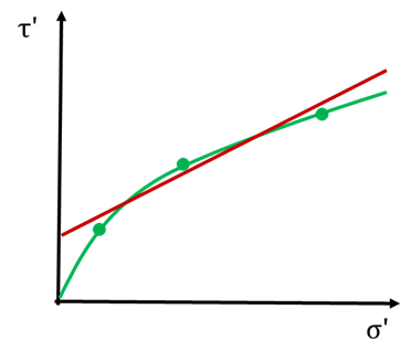
Figure 5 illustrates the errors implicit in the linear Mohr-Coulomb envelope. There are three data points obtained from a set of three triaxial or shear tests that define a non-linear failure curve and a linear Mohr-Coulomb envelope has been fitted through them. There is a mid-range of stress for which the soil strength is greater than that given by the linear Mohr-Coulomb criterion but at larger and smaller stresses the linear envelope is above the true curved envelope and it is unsafe. At small stresses relevant to stability of shallow landslides the errors using the linear Mohr-Coulomb envelope can be considerable (Atkinson, 2007, Atkinson and Crabb 1991).
2 SOIL STIFFNESS
2.1 Linear and non-linear stiffness
Stiffness is the relationship between changes of stress and changes of strain and stiffness modulus is the gradient of a stress- strain curve. These may be shear stress and strain giving a shear modulus G’ or mean stress and volumetric strain giving a bulk modulus K’ or a one-dimensional modulus M’. Figure 6(a) illustrates a general non-linear stress – strain curve. The stiffness at a point may be described as a tangent modulus δσ’/δε or as a secant modulus Δσ’/Δε.
Materials may be elastic or in-elastic and the criterion is what happens during a loading – unloading cycle. Elastic materials are conservative so (by definition) stress-strain curves for loading followed by unloading must be identical so no work is dissipated over the cycle as illustrated in Figure 6(b). Figure 6(c) illustrates the behaviour of a material that is linear but inelastic; the area within the loading – unloading loop is a measure of the work dissipated.
(a) Increments
(b) Non-linear elastic
(c) Linear inelastic
Figure 6: Material stiffness.


2.2 Conventional linear soil stiffness
Fig 7(a) illustrates a typical stress – strain curve of soil in a drained shear test with an unloading – reloading cycle. The stress – strain curve for a drained triaxial test would be similar. The gradient is the shear modulus G’ and for a triaxial test it is Young’s modulus E’. Fig 7(b) illustrates a typical stress – strain curve of soil in isotropic compression with an unloading – reloading cycle. The curve for one-dimensional compression would be similar. The gradient of the isotropic loading stress – strain curve is the bulk modulus K’ and for one-dimensional loading it is M’ = 1/mv where mv is the 1D compressibility.
(a)
(b)
Figure 7: Typical stress – strain curves for soil
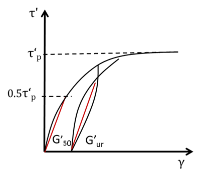
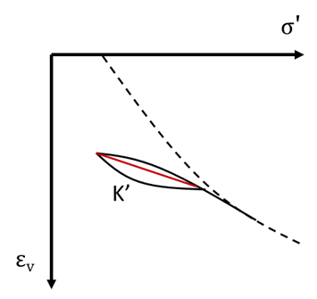
In conventional practice ground movements are calculated assuming the soil to be linear with a single value for stiffness. There are several ways in which the value of stiffness is determined and the red lines illustrate some of these.
2.3 Non-linear soil stiffness and settlements of foundations
For any of the loading or unloading stress – strain curves shown in Figure 7 the stiffness decays with strain from the start of the loading or unloading stage. The decay of stiffness with strain is well-established (Atkinson 2000) and a typical stiffness decay curve is illustrated in Figure 8. The strains vary over several orders of magnitude from very small strain (<0.001%) to large strain (>1%). Different experimental techniques are required to measure soil stiffness over different ranges of strain as illustrated in Figure 8.
Figure 8: Measurement of soil stiffness
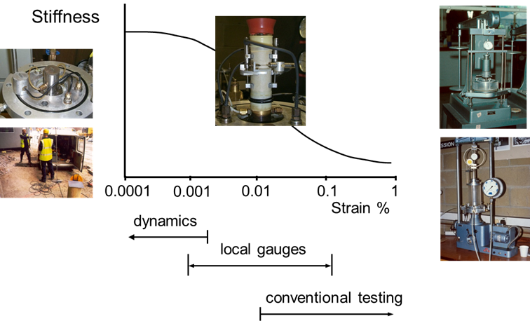
In conventional triaxial or oedometer tests there several sources of error in measurement of strain and it is impossible to obtain reliable measurements smaller than about 0.01%. To measure smaller strains it is necessary to use local gauges attached to the sample but these are limited to strains of about 0.001%. Soil stiffness at very small strain less than about 0.001% may be found from measurements of shear wave velocity in the ground or in laboratory samples.
2.4 Calculation of settlements of foundations
Some soils in the ground are heavily overconsolidated and are relatively stiff while other soils are lightly overconsolidated and are relatively soft. Analyses of settlements on soft soil should be treated differently from analyses of settlements on stiff soil. In practice there are two general cases and these are illustrated in Fig 9.
Buildings and embankments apply similar bearing pressures, typically 100 to 200kPa. An embankment can tolerate relatively large settlements of 100mm or more and can be built on soft soil. If the depth of soft soil is 10m the strains are of the order of 1%. Most buildings can tolerate only relatively small settlements of the order of 10mm and for a foundation 10m wide the mean strains are of the order of 0.1%. Shallow foundations can only be built on stiff soil so buildings on soft soil are most often on piled foundations.
The strains resulting from the same loading ∆σ’ are illustrated in Fig 9(c) and the corresponding stiffness decay curves are illustrated in Fig 9(d). The initial state of the soft soil is close to the normal consolidation line so the embankment loading moves the state from lightly overconsolidated to normally consolidated. The initial state of the stiff soil is far from the normal consolidation line and the state remains overconsolidated throughout the foundation loading.
(a)
(b)
(c)
(d)
Figure 9: Settlement of structures on stiff and soft soil


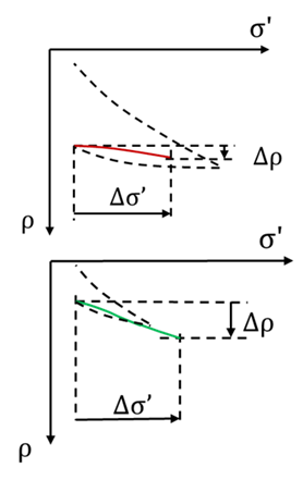
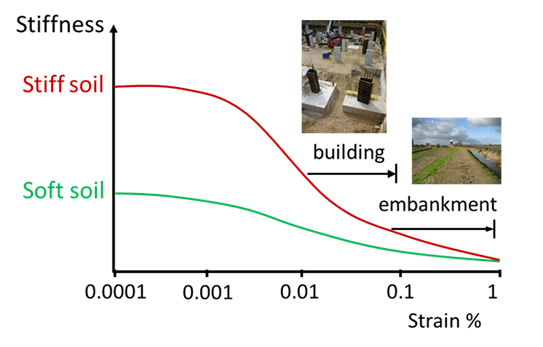
Figure 10 illustrates an embankment on a layer of soft soil of limited thickness. The deformations approximate to one-dimensional. The soil state moves from an initial lightly overconsolidated state and ends at a normally consolidated state. Over this range the stress – strain can reasonably be approximate as linear with gradient M’
(a)
(b)
Figure 10: Settlement of an embankment on soft soil
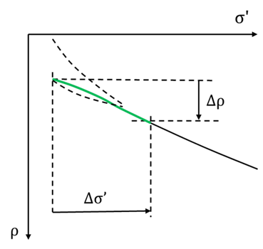

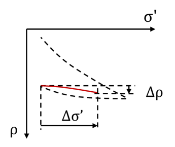
Figure 11(a) shows a foundation on stiff soil and Figure 11(b) shows the load –settlement curve. The state remains inside the normal consolidation line and the soil remains overconsolidated. A typical design would require settlements less than 10mm and for a foundation 10m wide this is a strain of about 0.1%. A typical stiffness – strain decay curve for stiff soil is illustrated in Figure 11(c). For very small strain less than about 0.001% the stiffness is approximately constant. For larger strains the stiffness decays and becomes very small as the soil fails. As a simplification, sufficient for routine foundation design, the decay of stiffness with log strain can be taken as linear as shown in Figure 11(d).
Values for E’0 the stiffness at very small strains less than about 0.001% can be found from routine measurements of shear wave velocity either in situ or from tests on laboratory samples. (Atkinson 2000). Stiff soils typically reach a state of failure with very small stiffness at strains approximately 1%. From Figure 11(d) the stiffness for simple design of a foundation on stiff soil can be taken as E’o/3 corresponding to settlements Δρ/B of 0.1%.
In routine ground engineering practice the errors implicit in these simplifications are often no greater than the uncertainties in determining the ground conditions and soil parameters from routine in situ or laboratory tests.
(a)
(b)
(c)
(d)
Figure 11: Settlement of a foundation on stiff soil


3 SUMMARY
In routine ground engineering practice soil strength is described by a linear Mohr-Coulomb criterion and stress-strain behaviour is linear. Neither of these approximations adequately represent the general features of soil behaviour.
Peak strengths of a variety or soils measured over range of normal stresses can be described by a simple power law given by equation 3 which is similar to the Hoek-Brown failure criterion for rocks.
The stress-strain behaviour of stiff soil is highly non-linear and stiffness decays rapidly with strain. A reasonable approximation is to take a design stiffness as E’o/3 corresponding to a strain of about 0.1%.
Strains below an embankment on soft soil are commonly of the order of 1% as the soil state moves from lightly overconsolidated to normally consolidated. Over this range the stress-strain behaviour approximates to linear with one-dimensional stiffness M’.
REFERENCES
Atkinson, J.H. (2000) 40th Rankine Lecture: Non-linear stiffness in routine design. Geotechnique; Vol. 50, No, 5, pp. 487-508
Atkinson, J.H. (2007) Peak strength of overconsolidated clays, Geotechnique, 57(2), 127-135.
Atkinson, J.H. and Crabb, G.I. (1991) Determination of Soil Strength Parameters for the Analysis of Highway Slope Failure. Proc. I.C.E. Int Conf. on Slope Stability Engineering Developments and Applications. Paper No 2, pp. 11-16.
Coulomb, C. A. (1773) Essai sur une application des regles de maximis et minimis a quelques problemes de statique relatifs a l’architecture. Mem. Div. Sav. Acad, Paris, Vol 7 pp 343-382
Heyman, J. (1972) Coulomb’s Memoir on Statics. Cambridge University Press.
Hoek E. and Brown E. T. (1980) Underground Excavations in Rock, p. 527. London, Inst Min Metall.
Terzaghi, K. (1936) The shearing resistance of saturated soil and the angle between the planes of shear. Proc. 1st Int. Conf. Soil Mech and Foundn Engng, Vol 1, pp 54-56, Harvard Mass.